Elements of Statistical Learning - Chapter 3 Partial Solutions
The second set of solutions is for Chapter 3, Linear Methods for Regression, covering linear regression models and extensions to least squares regression techniques, such as ridge regression, lasso, and least-angle regression.
Exercise Solutions
See the solutions in PDF format (source) for a more pleasant reading experience. This webpage was created from the LaTeX source using the LaTeX2Markdown utility - check it out on GitHub.
Exercise 3.1
Show that the $F$ statistic for dropping a single coefficient from a model is equal to the square of the corresponding $z$-score.
Proof
Recall that the $F$ statistic is defined by the following expression [ \frac{(RSS_0 - RSS_1) / (p_1 - p_0)}{RSS_1 / (N - p_1 - 1)}. ] where $RSS_0, RSS_1$ and $p_0 + 1, p_1 + 1$ refer to the residual sum of squares and the number of free parameters in the smaller and bigger models, respectively. Recall also that the $F$ statistic has a $F_{p_1 - p_0, N-p_1 - 1}$ distribution under the null hypothesis that the smaller model is correct.
Next, recall that the $z$-score of a coefficient is [ z_j = \frac{\hat \beta_j}{\hat \sigma \sqrt{v_j}} ] and under the null hypothesis that $\beta_j$ is zero, $z_j$ is distributed according to a $t$-distribution with $N-p-1$ degrees of freedom.
Hence, by dropping a single coefficient from a model, our $F$ statistic has a $F_{1, N-p - 1}$ where $p + 1$ are the number of parameters in the original model. Similarly, the corresponding $z$-score is distributed according to a $t_{N-p-1}$ distribution, and thus the square of the $z$-score is distributed according to an $F_{1, N-p-1}$ distribution, as required.
Thus both the $z$-score and the $F$ statistic test identical hypotheses under identical distributions. Thus they must have the same value in this case.
Exercise 3.2
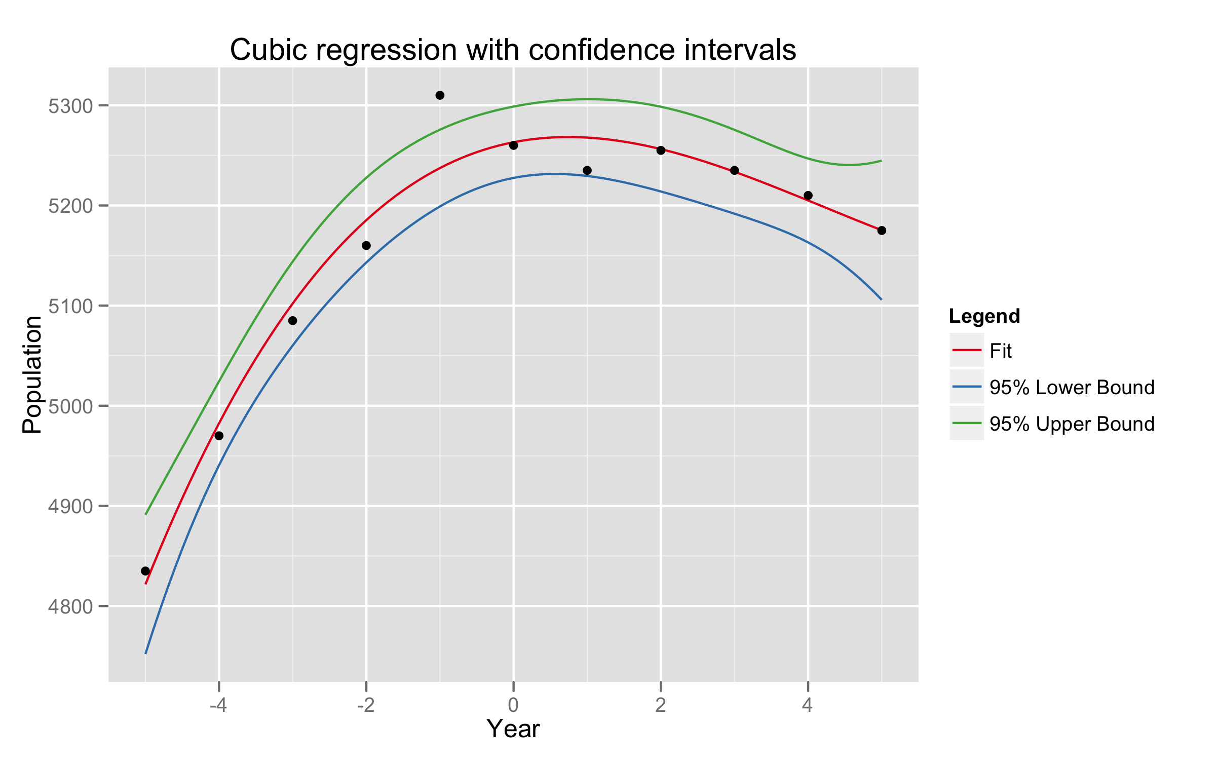
Given data on two variables $X$ and $Y$, consider fitting a cubic polynomial regression model $f(X) = \sum_{j=0}^{3} \beta_j X^j$. In addition to plotting the fitted curve, you would like a 95% confidence band about the curve. Consider the following two approaches:
- At each point $x_0$, form a 95% confidence interval for the linear function $a^T \beta = \sum_{j=0}^{3}\beta_j x_0^j$.
- Form a 95% confidence set for $\beta$ as in (3.15), which in tun generates confidence intervals for $f(x_0)$.
How do these approaches differ? Which band is likely to be wider? Conduct a small simulation experiment to compare the two methods.
Proof
The key distinction is that in the first case, we form the set of points such that we are 95% confident that $\hat f(x_0)$ is within this set, whereas in the second method, we are 95% confident that an arbitrary point is within our confidence interval. This is the distinction between a pointwise approach and a global confidence estimate.
In the pointwise approach, we seek to estimate the variance of an individual prediction - that is, to calculate $\text{Var}(\hat f(x_0) | x_0)$. Here, we have \begin{align} \sigma_0^2 = \text{Var}(\hat f(x_0) | x_0) &= \text{Var}(x_0^T \hat \beta | x_0) \\ &= x_0^T \text{Var}(\hat \beta) x_0 \\ &= \hat \sigma^2 x_0^T (X^T X)^{-1} x_0. \end{align} where $\hat \sigma^2$ is the estimated variance of the innovations $\epsilon_i$.
R code and graphs of the simulation are attached.
library('ProjectTemplate')
load.project()

# Raw data
simulation.xs <- c(1959, 1960, 1961, 1962, 1963, 1964, 1965, 1966, 1967, 1968, 1969)
simulation.ys <- c(4835, 4970, 5085, 5160, 5310, 5260, 5235, 5255, 5235, 5210, 5175)
simulation.df <- data.frame(pop = simulation.ys, year = simulation.xs)

# Rescale years
simulation.df$year = simulation.df$year - 1964

# Generate regression, construct confidence intervals
fit <- lm(pop ~ year + I(year^2) + I(year^3), data=simulation.df)
xs = seq(-5, 5, 0.1)
fit.confidence = predict(fit, data.frame(year=xs), interval="confidence", level=0.95)


# Create data frame containing variables of interest
df = as.data.frame(fit.confidence)
df$year <- xs
df = melt(df, id.vars="year")

p <- ggplot() + geom_line(aes(x=year, y=value, colour=variable), df) +
                geom_point(aes(x=year, y=pop), simulation.df)
p <- p + scale_x_continuous('Year') + scale_y_continuous('Population')
p <- p + opts(title="Cubic regression with confidence intervals")
p <- p + scale_color_brewer(name="Legend",
                            labels=c("Fit",
                                     "95% Lower Bound",
                                     "95% Upper Bound"),
                            palette="Set1")
ggsave(file.path('graphs', 'exercise_3_2.pdf'))
ggsave(file.path('graphs', 'exercise_3_2.png'), width=8, height=5, dpi=300)
TODO: Part 2.
Exercise 3.3 (The Gauss-Markov Theorem)
Prove the Gauss-Markov theorem: the least squares estimate of a parameter $a^T\beta$ has a variance no bigger than that of any other linear unbiased estimate of $a^T\beta$.
Secondly, show that if $\hat V$ is the variance-covariance matrix of the least squares estimate of $\beta$ and $\tilde V$ is the variance covariance matrix of any other linear unbiased estimate, then $\hat V \leq \tilde V$, where $B \leq A$ if $A - B$ is positive semidefinite.
Proof
Let $\hat \theta = a^T \hat \beta = a^T(X^TX)^{-1}X^T y$ be the least squares estimate of $a^T \beta$. Let $\tilde \theta = c^T y$ be any other unbiased linear estimator of $a^T \beta$. Now, let $d^T = c^T - a^T(X^{-1}X)^{-1}X^T$. Then as $c^T y$ is unbiased, we must have \begin{align} E(c^T y) &= E\left( a^T(X^{T}X)^{-1}X^T + d^T\right) y \\ &= a^T\beta + d^T X\beta \\ &= a^T\beta \end{align} as $c^T y$ is unbiased, which implies that $d^T X = 0$.
Now we calculate the variance of our estimator. We have \begin{align} \text{Var}(c^T y) &= c^T \text{Var}(y) c \\ &= \sigma^2 c^T c \\ &= \sigma^2 \left( a^T(X^{T}X)^{-1}X^T + d^T \right) \left( a^T (X^T X)^{-1} X^T + d^T \right)^T \\ &= \sigma^2 \left( a^T (X^T X)^{-1}X^T + d^T\right) \left(X (X^{T}X)^{-1}a + d\right) \\ &= \sigma^2 \left( a^T (X^TX)^{-1}X^T X(X^T X)^{-1} a + a^T (X^T X)^{-1} \underbrace{X^T d}_{=0} + \underbrace{d^T X}_{=0}(X^T X)^{-1} a + d^T d \right) \\ &= \sigma^2 \left(\underbrace{a^T (X^T X)^{-1} a}_{\text{Var}(\hat \theta)} + \underbrace{d^t d}_{\geq 0} \right) \end{align}
Thus $\text{Var}(\hat \theta) \leq \text{Var}(\tilde \theta)$ for all other unbiased linear estimators $\tilde \theta$.
The proof of the matrix version is almost identical, except we replace our vector $d$ with a matrix $D$. It is then possible to show that $\tilde V = \hat V + D^T D$, and as $D^T D$ is a positive semidefinite matrix for any $D$, we have $\hat V \leq \tilde V$.
Exercise 3.4
Show how the vector of least square coefficients can be obtained from a single pass of the Gram-Schmidt procedure. Represent your solution in terms of the QR decomposition of $X$.
Proof
Recall that by a single pass of the Gram-Schmidt procedure, we can write our matrix $X$ as [ X = Z \Gamma, ] where $Z$ contains the orthogonal columns $z_j$, and $\Gamma$ is an upper-diagonal matrix with ones on the diagonal, and $\gamma_{ij} = \frac{\langle z_i, x_j \rangle}{\| z_i \|^2}$. This is a reflection of the fact that by definition, [ x_j = z_j + \sum_{k=0}^{j-1} \gamma_{kj} z_k. ]
Now, by the $QR$ decomposition, we can write $X = QR$, where $Q$ is an orthogonal matrix and $R$ is an upper triangular matrix. We have $Q = Z D^{-1}$ and $R = D\Gamma$, where $D$ is a diagonal matrix with $D_{jj} = \| z_j \|$.
Now, by definition of $\hat \beta$, we have [ (X^T X) \hat \beta = X^T y. ] Now, using the $QR$ decomposition, we have \begin{align} (R^T Q^T) (QR) \hat \beta &= R^T Q^T y \\ R \hat \beta &= Q^T y \end{align} As $R$ is upper triangular, we can write \begin{align} R_{pp} \hat \beta_p &= \langle q_p, y \rangle \\ \| z_p \| \hat \beta_p &= \| z_p \|^{-1} \langle z_p, y \rangle \\ \hat \beta_p &= \frac{\langle z_p, y \rangle}{\| z_p \|^2} \end{align} in accordance with our previous results. Now, by back substitution, we can obtain the sequence of regression coefficients $\hat \beta_j$. As an example, to calculate $\hat \beta_{p-1}$, we have \begin{align} R_{p-1, p-1} \hat \beta_{p-1} + R_{p-1,p} \hat \beta_p &= \langle q_{p-1}, y \rangle \\ \| z_{p-1} \| \hat \beta_{p-1} + \| z_{p-1} \| \gamma_{p-1,p} \hat \beta_p &= \| z_{p-1} \|^{-1} \langle z_{p-1}, y \rangle \end{align} and then solving for $\hat \beta_{p-1}$. This process can be repeated for all $\beta_j$, thus obtaining the regression coefficients in one pass of the Gram-Schmidt procedure.
Exercise 3.5
Consider the ridge regression problem (3.41). Show that this problem is equivalent to the problem [ \hat \beta^c = \text{argmin}_{\beta^c} \left( \sum_{i=1}^{N} \left( y_i - \beta^c_0 - \sum_{j=1}^{p}(x_{ij} - \hat x_j) \beta^c_j \right)^2 + \lambda \sum_{j=1}^{p}{\beta_j^c}^2 \right)^2. ]
Proof
Consider rewriting our objective function above as [ L(\beta^c) = \sum_{i=1}^{N}\left(y_i - \left(\beta_0^c - \sum_{j=1}^{p} \bar x_j \beta_j^c \right) - \sum_{j=1}^p x_{ij} \beta_j^c \right)^2 + \lambda \sum_{j=1}^p {\beta_j^2}^2 ] Note that making the substitutions \begin{align} \beta_0 &\mapsto \beta_0^c - \sum_{j=1}^p \hat x_j \beta_j \\ \beta_j &\mapsto \beta^c_j, j = 1, 2, \dots, p \end{align} that $\hat \beta$ is a minimiser of the original ridge regression equation if $\hat \beta^c$ is a minimiser of our modified ridge regression.
The modified solution merely has a shifted intercept term, and all other coefficients remain the same.
Exercise 3.6
Show that the ridge regression estimate is the mean (and mode) of the posterior distribution, under a Gaussian prior $\beta \sim N(0, \tau \mathbf{I})$, and Gaussian sampling model $y \sim N(X \beta, \sigma^2 \mathbf{I})$. Find the relationship between the regularization parameter $\lambda$ in the ridge formula, and the variances $\tau$ and $\sigma^2$.
Exercise 3.7
Assume [ y_i \sim N(\beta_0 + x_i^T \beta, \sigma^2), i = 1, 2, \dots, N ] and the parameters $\beta_j$ are are each distributed as $N(0, \tau^2)$, independently of one another. Assume $\sigma^2$ and $\tau^2$ are known, show that the minus log-posterior density of $\beta$ is proportional to [ \sum_{i=1}^N \left( y_i - \beta_0 - \sum_{j=1}^p x_{ij} \beta_j \right)^2 + \lambda \sum_{j=1}^p \beta_j^2 ] where $\lambda = \frac{\sigma^2}{\tau^2}$.
Exercise 3.8
Consider the $QR$ decomposition of the uncentred $N \times (p+1)$ matrix $X$, whose first column is all ones, and the SVD of the $N \times p$ centred matrix $\tilde X$. Show that $Q_2$ and $U$ share the same subspace, where $Q_2$ is the submatrix of $Q$ with the first column removed. Under what circumstances will they be the same, up to sign flips?
Proof
Denote the columns of $X$ by $x_0, \dots, x_{p}$, the columns of $Q$ by $z_0, \dots, z_p$, the columns of $\tilde X$ by $\tilde x_1, \dots, x_n$, and the columns of $U$ by $u_1, \dots, u_p$. Without loss of generality, we can assume that for all $i$, $\| x_i \| = 1$ and that $X$ is non-singular (this cleans up the proof somewhat).
First, note that by the QR decomposition, we have that $\text{span}(x_0, \dots, x_j) = \text{span}(z_0, \dots, z_j)$ for any $0 \leq j \leq p$.
By our assumption, we have that $\tilde x_i = x_i - \bar x_i \mathbf{1}$ for $i = 1, \dots, p$. Thus we can write $\tilde x_i = \sum_{j \leq i} \alpha_j z_j$, and as the $z_j$ are orthogonal, we must be able to write $\tilde x_i$ in terms of $z_j$ for $j = 1, 2, \dots, i$. Thus $\text{span}(\tilde x_1, \dots, \tilde x_i) = \text{span}(z_1, \dots, z_i)$.
Finally, we calculate $\text{span}(u_1, \dots, u_p)$. We have that $U$ is a unitary $N \times p$ matrix, and thus the columns of $U$ span the column space of $\tilde X$, and thus the span of $Q_2$ is equal to the span of $U$.
TODO: When is $Q_2$ equal to $U$ up to parity? Is it where columns of
Exercise 3.9 (Forward stepwise regression)
Suppose that we have the $QR$ decomposition for the $N \times q$ matrix $X_1$ in a multiple regression problem with response $y$, and we have an additional $p - q$ predictors in matrix $X_2$. Denote the current residual by $r$. We wish to establish which one of these additional variables will reduce the residual-sum-of-squares the most when included with those in $X_1$. Describe an efficient procedure for doing this.
Proof
Select the vector $x_{j’}$ where \begin{align} x_{j’} = \text{argmin}_{j = q+1, \dots, p} \left| \left\langle \frac{x_q}{\| x_q \|}, r \right\rangle \right| \end{align}
This selects the vector that explains the maximal amount of variance in $r$ given $X_1$, and thus reduces the residual sum of squares the most. It is then possible to repeat this procedure by updating $X_2$ as in Algorithm 3.1.
Exercise 3.10 (Backward stepwise regression)
Suppose that we have the multiple regression fit of $y$ on $X$, along with standard errors and $z$-scores. We wish to establish which variable, when dropped, will increase the RSS the least. How would you do this?
Proof
By Exercise 3.1, we can show that the F-statistic for dropping a single coefficient from a model is equal to the square of the corresponding $z$-score. Thus, we drop the variable that has the lowest squared $z$-score from the model.
Exercise 3.11
Show that the solution to the multivariate linear regression problem (3.40) is given by (3.39). What happens if the covariance matrices $\Sigma_i$ are different for each observation?
Exercise 3.12
Show that the ridge regression estimates can be obtained by OLS on an augmented data set. We augment the centred matrix $X$ with $p$ additional rows $\sqrt{\lambda} \mathbf{I}$, and augment $y$ with $p$ zeroes.
Proof
For our augmented matrix $X_1$, equal to appending $\sqrt{\lambda I}$ to the original observation matrix $X$, we have that the $RSS$ expression for OLS regression becomes \begin{align} RSS &= \sum_{i=1}^{N+p} \left(y_i - \sum_{j=1}^p x_{ij} \beta_j \right)^2 \\ &= \sum_{i=1}^{N} \left( y_i - \sum_{j=1}^p x_{ij} \beta_j \right)^2 + \sum_{i = N + 1}^{N+p} \left(\sum_{j=1}^p x_{ij} \beta_j \right)^2 \\ &= \sum_{i=1}^{N} \left( y_i - \sum_{j=1}^p x_{ij} \beta_j \right)^2 + \sum_{j=1}^p \lambda \beta_j^2 \end{align} which is the objective function for the ridge regression estimate.
Exercise 3.13
Derive expression (3.62), and show that $\hat \beta^{\text{pcr}}(p) = \hat \beta^{\text{ls}}$.
Exercise 3.14
Show that in the orthogonal case, PLS stops after $m=1$ steps, because subsequent $\hat \phi_{mj}$ in step 2 in Algorithm 3.3 are zero.
Exercise 3.15
Verity expression (3.64), and hence show that the PLS directions are a compromise between the OLS coefficients and the principal component directions.
Exercise 3.16
Derive the entries in Table 3.4, the explicit forms for estimators in the orthogonal case.
Exercise 3.17
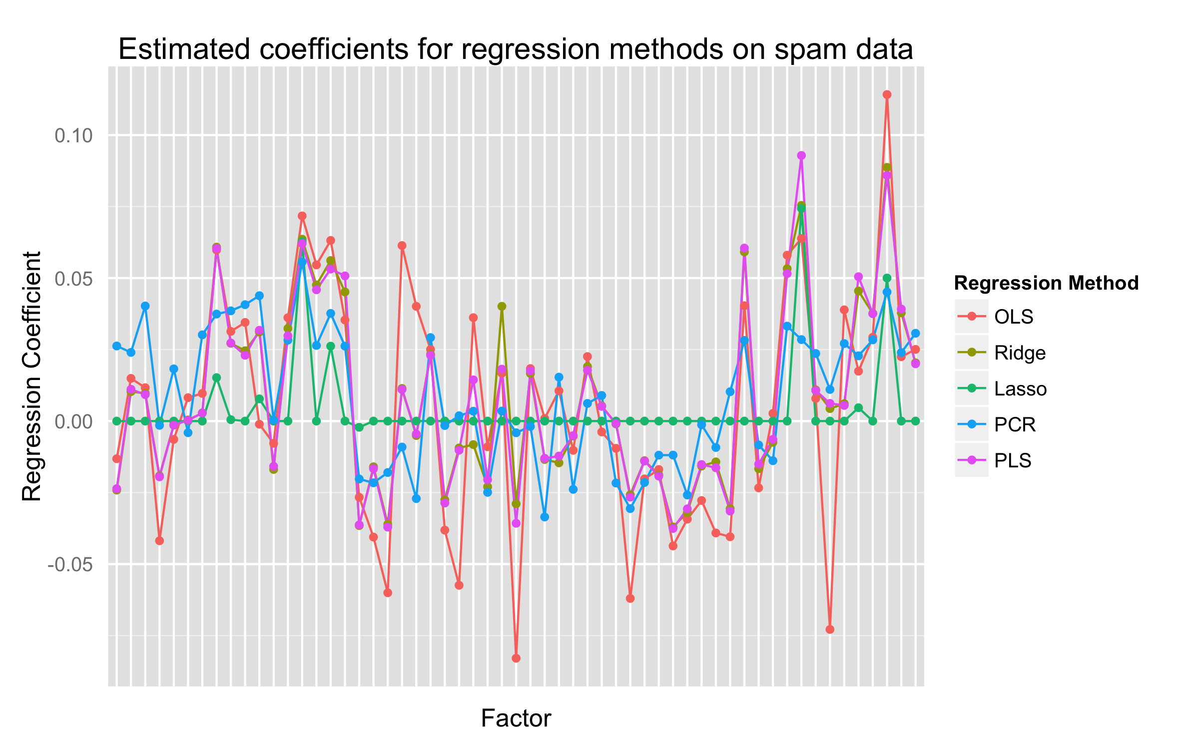
Repeat the analysis of Table 3.3 on the spam data discussed in Chapter 1.
Proof
R code implementing this method is attached. We require the MASS, lars, and pls packages.
library("ProjectTemplate")
load.project()

library("lars") # For least-angle and lasso
library("MASS") # For ridge
library("pls") # For PLS and PCR

mod.ls <- lm(Y ~ . - 1, spam.train)
mod.ridge <- lm.ridge(Y ~ ., spam.train)
mod.pcr <- pcr(formula=Y ~ ., data=spam.train, validation="CV")
mod.plsr <- plsr(formula=Y ~ ., data=spam.train, validation="CV")
mod.lars <- lars(as.matrix(spam.train[,1:ncol(spam.train) - 1]),
                 spam.train[,ncol(spam.train)],
                 type="lar")
mod.lasso <- lars(as.matrix(spam.train[,1:ncol(spam.train) - 1]),
                 spam.train[,ncol(spam.train)],
                 type="lasso")

mods.coeffs <- data.frame(ls=mod.ls$coef,
                          ridge=mod.ridge$coef,
                          lasso=mod.lasso$beta[10,],
                          pcr=mod.pcr$coef[,,10],
                          plsr=mod.plsr$coef[,,10]
                          )

mods.coeffs$xs = row.names(mods.coeffs)
plot.data <- melt(mods.coeffs, id="xs")

ggplot(data=plot.data,
       aes(x=factor(xs),
           y=value,
           group=variable,
           colour=variable)) +
        geom_line() +
        geom_point() +
        xlab("Factor") +
        ylab("Regression Coefficient") +
        opts(title = "Estimated coefficients for regression methods on spam data",
             axis.ticks = theme_blank(),
             axis.text.x = theme_blank()) +
        scale_colour_hue(name="Regression Method",
                         labels=c("OLS",
                                  "Ridge",
                                  "Lasso",
                                  "PCR",
                                  "PLS")
                         )

ggsave(file.path('graphs', 'exercise_3_17.pdf'))
ggsave(file.path('graphs', 'exercise_3_17.png'), width=8, height=5, dpi=300)